Simple Parallel (Tank Circuit) Resonance :-

 

Resonance in a Tank Circuit :-

A condition of resonance will be experienced in a tank circuit when the reactance of the capacitor and inductor are equal to each other. Because inductive reactance increases with increasing frequency and capacitive reactance decreases with increasing frequency, there will only be one frequency where these two reactances will be equal. Example:

 

Simple parallel resonant circuit (tank circuit).

 

In the above circuit, we have a 10 µF capacitor and a 100 mH inductor. Since we know the equations for determining the reactance of each at a given frequency, and we’re looking for that point where the two reactances are equal to each other, we can set the two reactance formula equal to each other and solve for frequency algebraically:

 

 

So there we have it: a formula to tell us the resonant frequency of a tank circuit, given the values of inductance (L) in Henrys and capacitance (C) in Farads. Plugging in the values of L and C in our example circuit, we arrive at a resonant frequency of 159.155 Hz.

Calculating Individual Impedances :-

What happens at resonance is quite interesting. With capacitive and inductive reactances equal to each other, the total impedance increases to infinity, meaning that the tank circuit draws no current from the AC power source!

We can calculate the individual impedances of the 10 µF capacitor and the 100 mH inductor and work through the parallel impedance formula to demonstrate this mathematically:

 

 

As you might have guessed, I chose these component values to give resonance impedances that were easy to work with (100 Ω even).

Parallel Impedance Formula :-

Now, we use the parallel impedance formula to see what happens to total Z:

 

 

SPICE Simulation Plot :-

We can’t divide any number by zero and arrive at a meaningful result, but we can say that the result approaches a value of infinity as the two parallel impedances get closer to each other.

What this means in practical terms is that, the total impedance of a tank circuit is infinite (behaving as an open circuit) at resonance. We can plot the consequences of this over a wide power supply frequency range with a short SPICE simulation.

 

 

Resonant circuit suitable for SPICE simulation.:-

 

The 1 pico-ohm (1 pΩ) resistor is placed in this SPICE analysis to overcome a limitation of SPICE: namely, that it cannot analyze a circuit containing a direct inductor-voltage source loop. (Figure below) A very low resistance value was chosen so as to have minimal effect on circuit behavior.

This SPICE simulation plots circuit current over a frequency range of 100 to 200 Hz in twenty even steps (100 and 200 Hz inclusive). Current magnitude on the graph increases from left to right, while frequency increases from top to bottom.

The current in this circuit takes a sharp dip around the analysis point of 157.9 Hz, which is the closest analysis point to our predicted resonance frequency of 159.155 Hz. It is at this point that total current from the power source falls to zero.

The “Nutmeg” Graphical Post-Processor Plot:-

The plot above is produced from the above spice circuit file ( *.cir), the command (.plot) in the last line producing the text plot on any printer or terminal. A better looking plot is produced by the “nutmeg” graphical post-processor, part of the spice package.

The above spice ( *.cir) does not require the plot (.plot) command, though it does no harm. The following commands produce the plot below:

 

spice -b -r resonant.raw resonant.cir 
 ( -b batch mode, -r raw file, input is resonant.cir)
 nutmeg resonant.raw

From the nutmeg prompt:

>setplot ac1 (setplot {enter} for list of plots)
 >display (for list of signals)
 >plot mag(v1#branch)
 (magnitude of complex current vector v1#branch)

 

Nutmeg produces plot of current I(v1) for parallel resonant circuit.

 

Bode Plots:-

Incidentally, the graph output produced by this SPICE computer analysis is more generally known as a Bode plot. Such graphs plot amplitude or phase shift on one axis and frequency on the other. The steepness of a Bode plot curve characterizes a circuit’s “frequency response,” or how sensitive it is to changes in frequency.

 

REVIEW:-

• Resonance occurs when capacitive and inductive reactances are equal to each other.
• For a tank circuit with no resistance (R), resonant frequency can be calculated with the following formula

• The total impedance of a parallel LC circuit approaches infinity as the power supply frequency approaches resonance.
• A Bode plot is a graph plotting waveform amplitude or phase on one axis and frequency on the other.

An Electric Pendulum :-

Capacitors store energy in the form of an electric field, and electrically manifest that stored energy as a potential: static voltage. Inductors store energy in the form of a magnetic field, and electrically manifest that stored energy as a kinetic motion of electrons: current.

Capacitors and inductors are flip-sides of the same reactive coin, storing and releasing energy in complementary modes. When these two types of reactive components are directly connected together, their complementary tendencies to store energy will produce an unusual result.

If either the capacitor or inductor starts out in a charged state, the two components will exchange energy between them, back and forth, creating their own AC voltage and current cycles.

If we assume that both components are subjected to a sudden application of voltage (say, from a momentarily connected battery), the capacitor will very quickly charge and the inductor will oppose change in current, leaving the capacitor in the charged state and the inductor in the discharged state.

 

Initial State :-

Capacitor charged: voltage at (+) peak; inductor discharged: zero current.

 

The capacitor will begin to discharge, its voltage decreasing. Meanwhile, the inductor will begin to build up a “charge” in the form of a magnetic field as current increases in the circuit.

 

Capacitor discharging: voltage decreasing; inductor charging: current increasing.

 

The inductor, still charging, will keep current flowing in the circuit until the capacitor has been completely discharged, leaving zero voltage across it.

 

Capacitor fully discharged: zero voltage; inductor fully charged: maximum current.

 

The inductor will maintain current flow even with no voltage applied. In fact, it will generate a voltage (like a battery) in order to keep current in the same direction. The capacitor, being the recipient of this current, will begin to accumulate a charge in the opposite polarity as before.

 

Capacitor charging: voltage increasing (in opposite polarity); inductor discharging: current decreasing.

 

When the inductor is finally depleted of its energy reserve and the electrons come to a halt, the capacitor will have reached full (voltage) charge in the opposite polarity as when it started.

 

Capacitor fully charged: voltage at (-) peak; inductor fully discharged: zero current.

 

Now we’re at a condition very similar to where we started: the capacitor at full charge and zero current in the circuit. The capacitor, as before, will begin to discharge through the inductor, causing an increase in current (in the opposite direction as before) and a decrease in voltage as it depletes its own energy reserve.

 

Capacitor discharging: voltage decreasing; inductor charging: current increasing.

 

Eventually the capacitor will discharge to zero volts, leaving the inductor fully charged with full current through it.

 

Capacitor fully discharged: zero voltage; inductor fully charged: current at (-) peak.

 

The inductor, desiring to maintain current in the same direction, will act like a source again, generating a voltage like a battery to continue the flow. In doing so, the capacitor will begin to charge up and the current will decrease in magnitude.

 

Capacitor charging: voltage increasing; inductor discharging: current decreasing.

 

Eventually the capacitor will become fully charged again as the inductor expends all of its energy reserves trying to maintain current. The voltage will once again be at its positive peak and the current at zero. This completes one full cycle of the energy exchange between the capacitor and inductor.

 

Capacitor fully charged: voltage at (+) peak; inductor fully discharged: zero current.

 

This oscillation will continue with steadily decreasing amplitude due to power losses from stray resistances in the circuit, until the process stops altogether.

Overall, this behavior is akin to that of a pendulum: as the pendulum mass swings back and forth, there is a transformation of energy taking place from kinetic (motion) to potential (height), in a similar fashion to the way energy is transferred in the capacitor/inductor circuit back and forth in the alternating forms of current (kinetic motion of electrons) and voltage (potential electric energy).

At the peak height of each swing of a pendulum, the mass briefly stops and switches directions. It is at this point that potential energy (height) is at a maximum and kinetic energy (motion) is at zero.

As the mass swings back the other way, it passes quickly through a point where the string is pointed straight down. At this point, potential energy (height) is at zero and kinetic energy (motion) is at maximum. Like the circuit, a pendulum’s back-and-forth oscillation will continue with a steadily dampened amplitude, the result of air friction (resistance) dissipating energy.

Also like the circuit, the pendulum’s position and velocity measurements trace two sine waves (90 degrees out of phase) over time.

 

Pendulum transfers energy between kinetic and potential energy as it swings low to high.

 

In physics, this kind of natural sine-wave oscillation for a mechanical system is called Simple Harmonic Motion (often abbreviated as “SHM”). The same underlying principles govern both the oscillation of a capacitor/inductor circuit and the action of a pendulum, hence the similarity in effect.

It is an interesting property of any pendulum that its periodic time is governed by the length of the string holding the mass, and not the weight of the mass itself. That is why a pendulum will keep swinging at the same frequency as the oscillations decrease in amplitude. The oscillation rate is independent of the amount of energy stored in it.

The same is true for the capacitor/inductor circuit. The rate of oscillation is strictly dependent on the sizes of the capacitor and inductor, not on the amount of voltage (or current) at each respective peak in the waves.

The ability for such a circuit to store energy in the form of oscillating voltage and current has earned it the name tank circuit. Its property of maintaining a single, natural frequency regardless of how much or little energy is actually being stored in it gives it special significance in electric circuit design.

However, this tendency to oscillate, or resonate, at a particular frequency is not limited to circuits exclusively designed for that purpose. In fact, nearly any AC circuit with a combination of capacitance and inductance (commonly called an “LC circuit”) will tend to manifest unusual effects when the AC power source frequency approaches that natural frequency.

This is true regardless of the circuit’s intended purpose.

If the power supply frequency for a circuit exactly matches the natural frequency of the circuit’s LC combination, the circuit is said to be in a state of resonance. The unusual effects will reach maximum in this condition of resonance.

For this reason, we need to be able to predict what the resonant frequency will be for various combinations of L and C, and be aware of what the effects of resonance are.

 

REVIEW :-

• A capacitor and inductor directly connected together form something called a tank circuit, which oscillates (or resonates) at one particular frequency. At that frequency, energy is alternately shuffled between the capacitor and the inductor in the form of alternating voltage and current 90 degrees out of phase with each other.
• When the power supply frequency for an AC circuit exactly matches that circuit’s natural oscillation frequency as set by the L and C components, a condition of resonance will have been reached.

AC Phase :-

Things start to get complicated when we need to relate two or more AC voltages or currents that are out of step with each other. By “out of step,” I mean that the two waveforms are not synchronized: that their peaks and zero points do not match up at the same points in time. The graph in figure below illustrates an example of this.

Out of phase waveforms.

 

The two waves shown above (A versus B) are of the same amplitude and frequency, but they are out of step with each other. In technical terms, this is called a phase shift. Earlier we saw how we could plot a “sine wave” by calculating the trigonometric sine function for angles ranging from 0 to 360 degrees, a full circle.

The starting point of a sine wave was zero amplitude at zero degrees, progressing to full positive amplitude at 90 degrees, zero at 180 degrees, full negative at 270 degrees, and back to the starting point of zero at 360 degrees. We can use this angle scale along the horizontal axis of our waveform plot to express how far out of step one wave is with another: Figure below

Wave A leads wave B by 45°

 

The shift between these two waveforms is about 45 degrees, the “A” wave being ahead of the “B” wave. A sampling of different phase shifts is given in the following graphs to better illustrate this concept: Figure below

Examples of phase shifts.

Because the waveforms in the above examples are at the same frequency, they will be out of step by the same angular amount at every point in time. For this reason, we can express phase shift for two or more waveforms of the same frequency as a constant quantity for the entire wave, and not just an expression of shift between any two particular points along the waves. That is, it is safe to say something like, “voltage ‘A’ is 45 degrees out of phase with voltage ‘B’.” Whichever waveform is ahead in its evolution is said to be leading and the one behind is said to be lagging.

Phase shift, like voltage, is always a measurement relative between two things. There’s really no such thing as a waveform with an absolute phase measurement because there’s no known universal reference for phase. Typically in the analysis of AC circuits, the voltage waveform of the power supply is used as a reference for phase, that voltage stated as “xxx volts at 0 degrees.” Any other AC voltage or current in that circuit will have its phase shift expressed in terms relative to that source voltage.

This is what makes AC circuit calculations more complicated than DC. When applying Ohm’s Law and Kirchhoff’s Laws, quantities of AC voltage and current must reflect phase shift as well as amplitude. Mathematical operations of addition, subtraction, multiplication, and division must operate on these quantities of phase shift as well as amplitude. Fortunately, there is a mathematical system of quantities called complex numbers ideally suited for this task of representing amplitude and phase.

Because the subject of complex numbers is so essential to the understanding of AC circuits, the next chapter will be devoted to that subject alone.

 

REVIEW :-

• Phase shift is where two or more waveforms are out of step with each other.
• The amount of phase shift between two waves can be expressed in terms of degrees, as defined by the degree units on the horizontal axis of the waveform graph used in plotting the trigonometric sine function.
• A leading waveform is defined as one waveform that is ahead of another in its evolution. A lagging waveform is one that is behind another. Example:

• Calculations for AC circuit analysis must take into consideration both amplitude and phase shift of voltage and current waveforms to be completely accurate. This requires the use of a mathematical system called complex numbers.

Simple AC Circuit Calculations :-

Over the course of the next few chapters, you will learn that AC circuit measurements and calculations can get very complicated due to the complex nature of alternating current in circuits with inductance and capacitance.

However, with simple circuits (figure below) involving nothing more than an AC power source and resistance, the same laws and rules of DC apply simply and directly.

AC circuit calculations for resistive circuits are the same as for DC.

 

 

Series resistances still add, parallel resistances still diminish, and the Laws of Kirchhoff and Ohm still hold true. Actually, as we will discover later on, these rules and laws always hold true, it’s just that we have to express the quantities of voltage, current, and opposition to current in more advanced mathematical forms.

With purely resistive circuits, however, these complexities of AC are of no practical consequence, and so we can treat the numbers as though we were dealing with simple DC quantities.

Because all these mathematical relationships still hold true, we can make use of our familiar “table” method of organizing circuit values just as with DC:

One major caveat needs to be given here: all measurements of AC voltage and current must be expressed in the same terms (peak, peak-to-peak, average, or RMS). If the source voltage is given in peak AC volts, then all currents and voltages subsequently calculated are cast in terms of peak units.

If the source voltage is given in AC RMS volts, then all calculated currents and voltages are cast in AC RMS units as well. This holds true for any calculation based on Ohm’s Laws, Kirchhoff’s Laws, etc. Unless otherwise stated, all values of voltage and current in AC circuits are generally assumed to be RMS rather than peak, average, or peak-to-peak.

In some areas of electronics, peak measurements are assumed, but in most applications (especially industrial electronics) the assumption is RMS.

 

REVIEW :-

• All the old rules and laws of DC (Kirchhoff’s Voltage and Current Laws, Ohm’s Law) still hold true for AC. However, with more complex circuits, we may need to represent the AC quantities in more complex form. More on this later, I promise!
• The “table” method of organizing circuit values is still a valid analysis tool for AC circuits.

Measurements of AC Magnitude :-

So far we know that AC voltage alternates in polarity and AC current alternates in direction. We also know that AC can alternate in a variety of different ways, and by tracing the alternation over time we can plot it as a “waveform.”

We can measure the rate of alternation by measuring the time it takes for a wave to evolve before it repeats itself (the “period”), and express this as cycles per unit time, or “frequency.” In music, frequency is the same as pitch, which is the essential property distinguishing one note from another.

However, we encounter a measurement problem if we try to express how large or small an AC quantity is. With DC, where quantities of voltage and current are generally stable, we have little trouble expressing how much voltage or current we have in any part of a circuit.

But how do you grant a single measurement of magnitude to something that is constantly changing?

Ways of Expressing the Magnitude of an AC Waveform :-

One way to express the intensity, or magnitude (also called the amplitude), of an AC quantity is to measure its peak height on a waveform graph. This is known as the peak or crest value of an AC waveform: Figure below

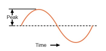
Peak voltage of a waveform.

 

Another way is to measure the total height between opposite peaks. This is known as the peak-to-peak (P-P) value of an AC waveform: Figure below

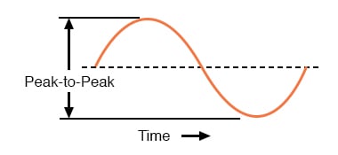
Peak-to-peak voltage of a waveform.

 

Unfortunately, either one of these expressions of waveform amplitude can be misleading when comparing two different types of waves. For example, a square wave peaking at 10 volts is obviously a greater amount of voltage for a greater amount of time than a triangle wave peaking at 10 volts.

The effects of these two AC voltages powering a load would be quite different: Figure below

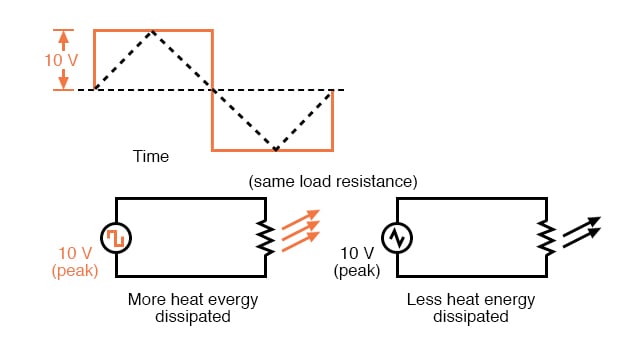
A square wave produces a greater heating effect than the same peak voltage triangle wave.

 

One way of expressing the amplitude of different wave shapes in a more equivalent fashion is to mathematically average the values of all the points on a waveform’s graph to a single, aggregate number. This amplitude measurement is known simply as the average value of the waveform.

If we average all the points on the waveform algebraically (that is, to consider their sign, either positive or negative), the average value for most waveforms is technically zero, because all the positive points cancel out all the negative points over a full cycle: Figure below

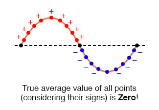
The average value of a sine wave is zero.

 

This, of course, will be true for any waveform having equal-area portions above and below the “zero” line of a plot. However, as a practical measure of a waveform’s aggregate value, “average” is usually defined as the mathematical mean of all the points’ absolute values over a cycle.

In other words, we calculate the practical average value of the waveform by considering all points on the wave as positive quantities, as if the waveform looked like this: Figure below

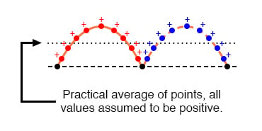
Waveform seen by AC “average responding” meter.

 

Polarity-insensitive mechanical meter movements (meters designed to respond equally to the positive and negative half-cycles of an alternating voltage or current) register in proportion to the waveform’s (practical) average value, because the inertia of the pointer against the tension of the spring naturally averages the force produced by the varying voltage/current values over time.

Conversely, polarity-sensitive meter movements vibrate uselessly if exposed to AC voltage or current, their needles oscillating rapidly about the zero mark, indicating the true (algebraic) average value of zero for a symmetrical waveform. When the “average” value of a waveform is referenced in this text, it will be assumed that the “practical” definition of average is intended unless otherwise specified.

Another method of deriving an aggregate value for waveform amplitude is based on the waveform’s ability to do useful work when applied to a load resistance. Unfortunately, an AC measurement based on work performed by a waveform is not the same as that waveform’s “average” value, because the power dissipated by a given load (work performed per unit time) is not directly proportional to the magnitude of either the voltage or current impressed upon it.

Rather, power is proportional to the square of the voltage or current applied to a resistance (P = E2/R, and P = I2R). Although the mathematics of such an amplitude measurement might not be straightforward, the utility of it is.

Consider a bandsaw and a jigsaw, two pieces of modern woodworking equipment. Both types of saws cut with a thin, toothed, motor-powered metal blade to cut wood. But while the bandsaw uses a continuous motion of the blade to cut, the jigsaw uses a back-and-forth motion.

The comparison of alternating current (AC) to direct current (DC) may be likened to the comparison of these two saw types: Figure below

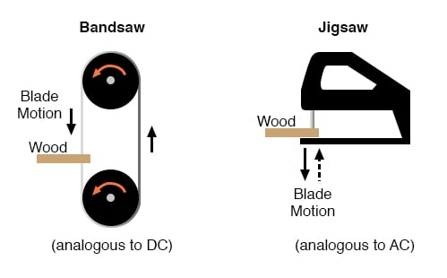
Bandsaw-jigsaw analogy of DC vs AC.

 

The problem of trying to describe the changing quantities of AC voltage or current in a single, aggregate measurement is also present in this saw analogy: how might we express the speed of a jigsaw blade? A bandsaw blade moves with a constant speed, similar to the way DC voltage pushes or DC current moves with a constant magnitude. A jigsaw blade, on the other hand, moves back and forth, its blade speed constantly changing. What is more, the back-and-forth motion of any two jigsaws may not be of the same type, depending on the mechanical design of the saws.

One jigsaw might move its blade with a sine-wave motion, while another with a triangle-wave motion. To rate a jigsaw based on its peak blade speed would be quite misleading when comparing one jigsaw to another (or a jigsaw with a bandsaw!). Despite the fact that these different saws move their blades in different manners, they are equal in one respect: they all cut wood, and a quantitative comparison of this common function can serve as a common basis for which to rate blade speed.

Picture a jigsaw and bandsaw side-by-side, equipped with identical blades (same tooth pitch, angle, etc.), equally capable of cutting the same thickness of the same type of wood at the same rate. We might say that the two saws were equivalent or equal in their cutting capacity. Might this comparison be used to assign a “bandsaw equivalent” blade speed to the jigsaw’s back-and-forth blade motion; to relate the wood-cutting effectiveness of one to the other?

This is the general idea used to assign a “DC equivalent” measurement to any AC voltage or current: whatever magnitude of DC voltage or current would produce the same amount of heat energy dissipation through an equal resistance: Figure below

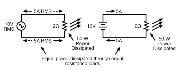
An RMS voltage produces the same heating effect as the same DC voltage

 

How is Root Mean Square (RMS) Relevant to AC? :-

In the two circuits above, we have the same amount of load resistance (2 Ω) dissipating the same amount of power in the form of heat (50 watts), one powered by AC and the other by DC. Because the AC voltage source pictured above is equivalent (in terms of power delivered to a load) to a 10 volt DC battery, we would call this a “10 volt” AC source.

More specifically, we would denote its voltage value as being 10 volts RMS. The qualifier “RMS” stands for Root Mean Square, the algorithm used to obtain the DC equivalent value from points on a graph (essentially, the procedure consists of squaring all the positive and negative points on a waveform graph, averaging those squared values, then taking the square root of that average to obtain the final answer).

Sometimes the alternative terms equivalent or DC equivalent are used instead of “RMS,” but the quantity and principle are both the same.

RMS amplitude measurement is the best way to relate AC quantities to DC quantities, or other AC quantities of differing waveform shapes, when dealing with measurements of electric power.

For other considerations, peak or peak-to-peak measurements may be the best to employ. For instance, when determining the proper size of wire (ampacity) to conduct electric power from a source to a load, RMS current measurement is the best to use, because the principal concern with current is overheating of the wire, which is a function of power dissipation caused by current through the resistance of the wire.

However, when rating insulators for service in high-voltage AC applications, peak voltage measurements are the most appropriate, because the principal concern here is insulator “flashover” caused by brief spikes of voltage, irrespective of time.

Instruments Used to Measure the Amplitude of a Waveform :-

Peak and peak-to-peak measurements are best performed with an oscilloscope, which can capture the crests of the waveform with a high degree of accuracy due to the fast action of the cathode-ray-tube in response to changes in voltage. For RMS measurements, analog meter movements (D’Arsonval, Weston, iron vane, electrodynamometer) will work so long as they have been calibrated in RMS figures.

Because the mechanical inertia and dampening effects of an electromechanical meter movement makes the deflection of the needle naturally proportional to the average value of the AC, not the true RMS value, analog meters must be specifically calibrated (or mis-calibrated, depending on how you look at it) to indicate voltage or current in RMS units.

The accuracy of this calibration depends on an assumed waveshape, usually a sine wave.

Electronic meters specifically designed for RMS measurement are best for the task. Some instrument manufacturers have designed ingenious methods for determining the RMS value of any waveform. One such manufacturer produces “True-RMS” meters with a tiny resistive heating element powered by a voltage proportional to that being measured.

The heating effect of that resistance element is measured thermally to give a true RMS value with no mathematical calculations whatsoever, just the laws of physics in action in fulfillment of the definition of RMS. The accuracy of this type of RMS measurement is independent of waveshape.

Relationship of Peak, Peak-to-Peak, Average, and RMS :-

For “pure” waveforms, simple conversion coefficients exist for equating Peak, Peak-to-Peak, Average (practical, not algebraic), and RMS measurements to one another: 

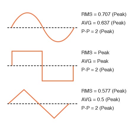
Conversion factors for common waveforms.

 

In addition to RMS, average, peak (crest), and peak-to-peak measures of an AC waveform, there are ratios expressing the proportionality between some of these fundamental measurements. The crest factor of an AC waveform, for instance, is the ratio of its peak (crest) value divided by its RMS value.

The form factor of an AC waveform is the ratio of its RMS value divided by its average value. Square-shaped waveforms always have crest and form factors equal to 1, since the peak is the same as the RMS and average values. Sinusoidal waveforms have an RMS value of 0.707 (the reciprocal of the square root of 2) and a form factor of 1.11 (0.707/0.636).

Triangle- and sawtooth-shaped waveforms have RMS values of 0.577 (the reciprocal of square root of 3) and form factors of 1.15 (0.577/0.5).

Bear in mind that the conversion constants shown here for peak, RMS, and average amplitudes of sine waves, square waves, and triangle waves hold true only for pure forms of these waveshapes. The RMS and average values of distorted waveshapes are not related by the same ratios: Figure below

Arbitrary waveforms have no simple conversions.

 

This is a very important concept to understand when using an analog D’Arsonval meter movement to measure AC voltage or current. An analog D’Arsonval movement, calibrated to indicate sine-wave RMS amplitude, will only be accurate when measuring pure sine waves.

If the waveform of the voltage or current being measured is anything but a pure sine wave, the indication given by the meter will not be the true RMS value of the waveform, because the degree of needle deflection in an analog D’Arsonval meter movement is proportional to the average value of the waveform, not the RMS.

RMS meter calibration is obtained by “skewing” the span of the meter so that it displays a small multiple of the average value, which will be equal to be the RMS value for a particular waveshape and a particular waveshape only.

Since the sine-wave shape is most common in electrical measurements, it is the waveshape assumed for analog meter calibration, and the small multiple used in the calibration of the meter is 1.1107 (the form factor: 0.707/0.636: the ratio of RMS divided by average for a sinusoidal waveform).

Any waveshape other than a pure sine wave will have a different ratio of RMS and average values, and thus a meter calibrated for sine-wave voltage or current will not indicate true RMS when reading a non-sinusoidal wave. Bear in mind that this limitation applies only to simple, analog AC meters not employing “True-RMS” technology.

 

REVIEW :-

• The amplitude of an AC waveform is its height as depicted on a graph over time. An amplitude measurement can take the form of peak, peak-to-peak, average, or RMS quantity.
• Peak amplitude is the height of an AC waveform as measured from the zero mark to the highest positive or lowest negative point on a graph. Also known as the crest amplitude of a wave.
• Peak-to-peak amplitude is the total height of an AC waveform as measured from maximum positive to maximum negative peaks on a graph. Often abbreviated as “P-P”.
• Average amplitude is the mathematical “mean” of all a waveform’s points over the period of one cycle. Technically, the average amplitude of any waveform with equal-area portions above and below the “zero” line on a graph is zero. However, as a practical measure of amplitude, a waveform’s average value is often calculated as the mathematical mean of all the points’ absolute values (taking all the negative values and considering them as positive). For a sine wave, the average value so calculated is approximately 0.637 of its peak value.
• “RMS” stands for Root Mean Square, and is a way of expressing an AC quantity of voltage or current in terms functionally equivalent to DC. For example, 10 volts AC RMS is the amount of voltage that would produce the same amount of heat dissipation across a resistor of given value as a 10 volt DC power supply. Also known as the “equivalent” or “DC equivalent” value of an AC voltage or current. For a sine wave, the RMS value is approximately 0.707 of its peak value.
• The crest factor of an AC waveform is the ratio of its peak (crest) to its RMS value.
• The form factor of an AC waveform is the ratio of its RMS value to its average value.
• Analog, electromechanical meter movements respond proportionally to the average value of an AC voltage or current. When RMS indication is desired, the meter’s calibration must be “skewed” accordingly. This means that the accuracy of an electromechanical meter’s RMS indication is dependent on the purity of the waveform: whether it is the exact same waveshape as the waveform used in calibrating.

Harmonic Phase Sequences :-

In the last section, we saw how the 3rd harmonic and all of its integer multiples (collectively called triplen harmonics) generated by 120° phase-shifted fundamental waveforms are actually in phase with each other.

In a 60 Hz three-phase power system, where phases A, B, and C are 120° apart, the third-harmonic multiples of those frequencies (180 Hz) fall perfectly into phase with each other.

This can be thought of in graphical terms, (figure below) and/or in mathematical terms:

 

Harmonic currents of Phases A, B, C all coincide, that is, no rotation.

 

Extended Mathematical Table with Odd-Numbered Harmonics

 

If we extend the mathematical table to include higher odd-numbered harmonics, we will notice an interesting pattern develop with regard to the rotation or sequence of the harmonic frequencies:

Harmonics such as the 7th, which “rotate” with the same sequence as the fundamental, are called positive sequence.

Harmonics such as the 5th, which “rotate” in the opposite sequence as the fundamental, are called negative sequence.

Triplen harmonics (3rd and 9th shown in this table) which don’t “rotate” at all because they’re in phase with each other, are called zero sequence.

This pattern of positive-zero-negative-positive continues indefinitely for all odd-numbered harmonics, lending itself to expression in a table like this: