Simple Parallel (Tank Circuit) Resonance :-

 

Resonance in a Tank Circuit :-

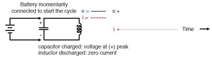
A condition of resonance will be experienced in a tank circuit when the reactance of the capacitor and inductor are equal to each other. Because inductive reactance increases with increasing frequency and capacitive reactance decreases with increasing frequency, there will only be one frequency where these two reactances will be equal. Example:

 

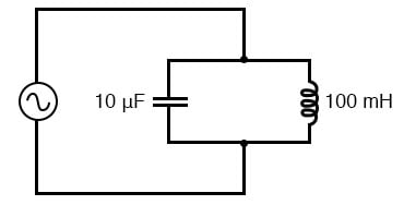
Simple parallel resonant circuit (tank circuit).

 

In the above circuit, we have a 10 µF capacitor and a 100 mH inductor. Since we know the equations for determining the reactance of each at a given frequency, and we’re looking for that point where the two reactances are equal to each other, we can set the two reactance formula equal to each other and solve for frequency algebraically:

 

 

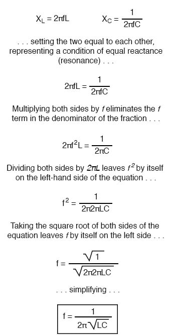
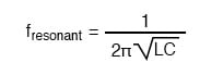
So there we have it: a formula to tell us the resonant frequency of a tank circuit, given the values of inductance (L) in Henrys and capacitance (C) in Farads. Plugging in the values of L and C in our example circuit, we arrive at a resonant frequency of 159.155 Hz.

Calculating Individual Impedances :-

What happens at resonance is quite interesting. With capacitive and inductive reactances equal to each other, the total impedance increases to infinity, meaning that the tank circuit draws no current from the AC power source!

We can calculate the individual impedances of the 10 µF capacitor and the 100 mH inductor and work through the parallel impedance formula to demonstrate this mathematically:

 

 

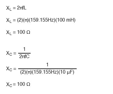
As you might have guessed, I chose these component values to give resonance impedances that were easy to work with (100 Ω even).

Parallel Impedance Formula :-

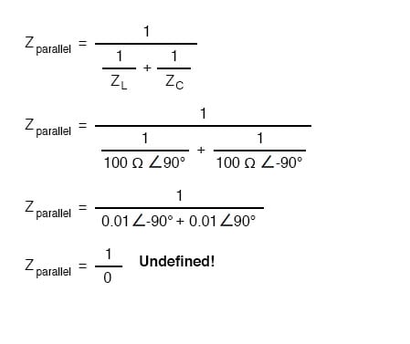
Now, we use the parallel impedance formula to see what happens to total Z:

 

 

SPICE Simulation Plot :-

We can’t divide any number by zero and arrive at a meaningful result, but we can say that the result approaches a value of infinity as the two parallel impedances get closer to each other.

What this means in practical terms is that, the total impedance of a tank circuit is infinite (behaving as an open circuit) at resonance. We can plot the consequences of this over a wide power supply frequency range with a short SPICE simulation.

 

 

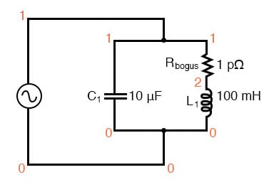
Resonant circuit suitable for SPICE simulation.:-

 

The 1 pico-ohm (1 pΩ) resistor is placed in this SPICE analysis to overcome a limitation of SPICE: namely, that it cannot analyze a circuit containing a direct inductor-voltage source loop. (Figure below) A very low resistance value was chosen so as to have minimal effect on circuit behavior.

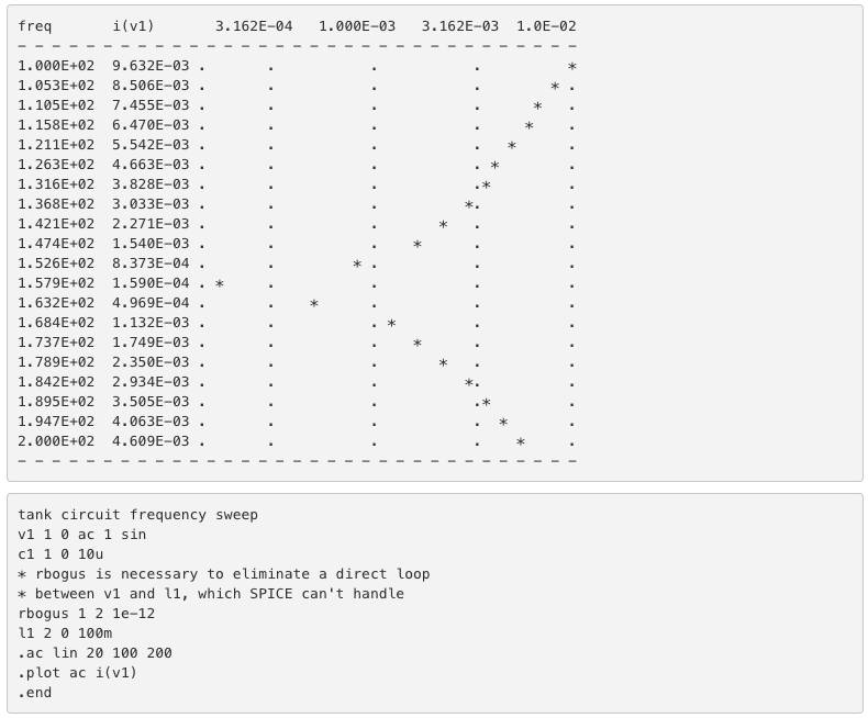
This SPICE simulation plots circuit current over a frequency range of 100 to 200 Hz in twenty even steps (100 and 200 Hz inclusive). Current magnitude on the graph increases from left to right, while frequency increases from top to bottom.

The current in this circuit takes a sharp dip around the analysis point of 157.9 Hz, which is the closest analysis point to our predicted resonance frequency of 159.155 Hz. It is at this point that total current from the power source falls to zero.

The “Nutmeg” Graphical Post-Processor Plot:-

The plot above is produced from the above spice circuit file ( *.cir), the command (.plot) in the last line producing the text plot on any printer or terminal. A better looking plot is produced by the “nutmeg” graphical post-processor, part of the spice package.

The above spice ( *.cir) does not require the plot (.plot) command, though it does no harm. The following commands produce the plot below:

 

spice -b -r resonant.raw resonant.cir 
 ( -b batch mode, -r raw file, input is resonant.cir)
 nutmeg resonant.raw

From the nutmeg prompt:

>setplot ac1 (setplot {enter} for list of plots)
 >display (for list of signals)
 >plot mag(v1#branch)
 (magnitude of complex current vector v1#branch)

 

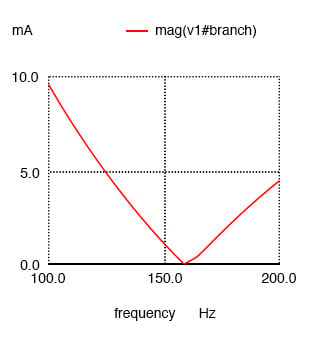
Nutmeg produces plot of current I(v1) for parallel resonant circuit.

 

Bode Plots:-

Incidentally, the graph output produced by this SPICE computer analysis is more generally known as a Bode plot. Such graphs plot amplitude or phase shift on one axis and frequency on the other. The steepness of a Bode plot curve characterizes a circuit’s “frequency response,” or how sensitive it is to changes in frequency.

 

REVIEW:-

• Resonance occurs when capacitive and inductive reactances are equal to each other.
• For a tank circuit with no resistance (R), resonant frequency can be calculated with the following formula

• The total impedance of a parallel LC circuit approaches infinity as the power supply frequency approaches resonance.
• A Bode plot is a graph plotting waveform amplitude or phase on one axis and frequency on the other.

An Electric Pendulum :-

Capacitors store energy in the form of an electric field, and electrically manifest that stored energy as a potential: static voltage. Inductors store energy in the form of a magnetic field, and electrically manifest that stored energy as a kinetic motion of electrons: current.

Capacitors and inductors are flip-sides of the same reactive coin, storing and releasing energy in complementary modes. When these two types of reactive components are directly connected together, their complementary tendencies to store energy will produce an unusual result.

If either the capacitor or inductor starts out in a charged state, the two components will exchange energy between them, back and forth, creating their own AC voltage and current cycles.

If we assume that both components are subjected to a sudden application of voltage (say, from a momentarily connected battery), the capacitor will very quickly charge and the inductor will oppose change in current, leaving the capacitor in the charged state and the inductor in the discharged state.

 

Initial State :-

Capacitor charged: voltage at (+) peak; inductor discharged: zero current.

 

The capacitor will begin to discharge, its voltage decreasing. Meanwhile, the inductor will begin to build up a “charge” in the form of a magnetic field as current increases in the circuit.

 

Capacitor discharging: voltage decreasing; inductor charging: current increasing.

 

The inductor, still charging, will keep current flowing in the circuit until the capacitor has been completely discharged, leaving zero voltage across it.

 

Capacitor fully discharged: zero voltage; inductor fully charged: maximum current.

 

The inductor will maintain current flow even with no voltage applied. In fact, it will generate a voltage (like a battery) in order to keep current in the same direction. The capacitor, being the recipient of this current, will begin to accumulate a charge in the opposite polarity as before.

 

Capacitor charging: voltage increasing (in opposite polarity); inductor discharging: current decreasing.

 

When the inductor is finally depleted of its energy reserve and the electrons come to a halt, the capacitor will have reached full (voltage) charge in the opposite polarity as when it started.

 

Capacitor fully charged: voltage at (-) peak; inductor fully discharged: zero current.

 

Now we’re at a condition very similar to where we started: the capacitor at full charge and zero current in the circuit. The capacitor, as before, will begin to discharge through the inductor, causing an increase in current (in the opposite direction as before) and a decrease in voltage as it depletes its own energy reserve.

 

Capacitor discharging: voltage decreasing; inductor charging: current increasing.

 

Eventually the capacitor will discharge to zero volts, leaving the inductor fully charged with full current through it.

 

Capacitor fully discharged: zero voltage; inductor fully charged: current at (-) peak.

 

The inductor, desiring to maintain current in the same direction, will act like a source again, generating a voltage like a battery to continue the flow. In doing so, the capacitor will begin to charge up and the current will decrease in magnitude.

 

Capacitor charging: voltage increasing; inductor discharging: current decreasing.

 

Eventually the capacitor will become fully charged again as the inductor expends all of its energy reserves trying to maintain current. The voltage will once again be at its positive peak and the current at zero. This completes one full cycle of the energy exchange between the capacitor and inductor.

 

Capacitor fully charged: voltage at (+) peak; inductor fully discharged: zero current.

 

This oscillation will continue with steadily decreasing amplitude due to power losses from stray resistances in the circuit, until the process stops altogether.

Overall, this behavior is akin to that of a pendulum: as the pendulum mass swings back and forth, there is a transformation of energy taking place from kinetic (motion) to potential (height), in a similar fashion to the way energy is transferred in the capacitor/inductor circuit back and forth in the alternating forms of current (kinetic motion of electrons) and voltage (potential electric energy).

At the peak height of each swing of a pendulum, the mass briefly stops and switches directions. It is at this point that potential energy (height) is at a maximum and kinetic energy (motion) is at zero.

As the mass swings back the other way, it passes quickly through a point where the string is pointed straight down. At this point, potential energy (height) is at zero and kinetic energy (motion) is at maximum. Like the circuit, a pendulum’s back-and-forth oscillation will continue with a steadily dampened amplitude, the result of air friction (resistance) dissipating energy.

Also like the circuit, the pendulum’s position and velocity measurements trace two sine waves (90 degrees out of phase) over time.

 

Pendulum transfers energy between kinetic and potential energy as it swings low to high.

 

In physics, this kind of natural sine-wave oscillation for a mechanical system is called Simple Harmonic Motion (often abbreviated as “SHM”). The same underlying principles govern both the oscillation of a capacitor/inductor circuit and the action of a pendulum, hence the similarity in effect.

It is an interesting property of any pendulum that its periodic time is governed by the length of the string holding the mass, and not the weight of the mass itself. That is why a pendulum will keep swinging at the same frequency as the oscillations decrease in amplitude. The oscillation rate is independent of the amount of energy stored in it.

The same is true for the capacitor/inductor circuit. The rate of oscillation is strictly dependent on the sizes of the capacitor and inductor, not on the amount of voltage (or current) at each respective peak in the waves.

The ability for such a circuit to store energy in the form of oscillating voltage and current has earned it the name tank circuit. Its property of maintaining a single, natural frequency regardless of how much or little energy is actually being stored in it gives it special significance in electric circuit design.

However, this tendency to oscillate, or resonate, at a particular frequency is not limited to circuits exclusively designed for that purpose. In fact, nearly any AC circuit with a combination of capacitance and inductance (commonly called an “LC circuit”) will tend to manifest unusual effects when the AC power source frequency approaches that natural frequency.

This is true regardless of the circuit’s intended purpose.

If the power supply frequency for a circuit exactly matches the natural frequency of the circuit’s LC combination, the circuit is said to be in a state of resonance. The unusual effects will reach maximum in this condition of resonance.

For this reason, we need to be able to predict what the resonant frequency will be for various combinations of L and C, and be aware of what the effects of resonance are.

 

REVIEW :-

• A capacitor and inductor directly connected together form something called a tank circuit, which oscillates (or resonates) at one particular frequency. At that frequency, energy is alternately shuffled between the capacitor and the inductor in the form of alternating voltage and current 90 degrees out of phase with each other.
• When the power supply frequency for an AC circuit exactly matches that circuit’s natural oscillation frequency as set by the L and C components, a condition of resonance will have been reached.

Some Examples with AC Circuits :-

Let’s connect three AC voltage sources in series and use complex numbers to determine additive voltages.

All the rules and laws learned in the study of DC circuits apply to AC circuits as well (Ohm’s Law, Kirchhoff’s Laws, network analysis methods), with the exception of power calculations (Joule’s Law).

The only qualification is that all variables must be expressed in complex form, taking into account phase as well as magnitude, and all voltages and currents must be of the same frequency (in order that their phase relationships remain constant). (Figure below)

 

KVL allows the addition of complex voltages.

 

The polarity marks for all three voltage sources are oriented in such a way that their stated voltages should add to make the total voltage across the load resistor.

Notice that although magnitude and phase angle is given for each AC voltage source, no frequency value is specified. If this is the case, it is assumed that all frequencies are equal, thus meeting our qualifications for applying DC rules to an AC circuit (all figures given in the complex form, all of the same frequency).

The setup of our equation to find total voltage appears as such:

 

 

Graphically, the vectors add up as shown in Figure below.

 

Graphic addition of vector voltages.

 

The sum of these vectors will be a resultant vector originating at the starting point for the 22-volt vector (the dot at upper-left of the diagram) and terminating at the ending point for the 15-volt vector (arrow tip at the middle-right of the diagram): (Figure below)

 

Resultant is equivalent to the vector sum of the three original voltages.

 

In order to determine what the resultant vector’s magnitude and angle are without resorting to graphical images, we can convert each one of these polar-form complex numbers into rectangular form and add.

Remember, we’re adding these figures together because the polarity marks for the three voltage sources are oriented in an additive manner:

 

 

In polar form, this equates to 36.8052 volts ∠ -20.5018°. What this means in real terms is that the voltage measured across these three voltage sources will be 36.8052 volts, lagging the 15 volts (0° phase reference) by 20.5018°.

A voltmeter connected across these points in a real circuit would only indicate the polar magnitude of the voltage (36.8052 volts), not the angle. An oscilloscope could be used to display two voltage waveforms and thus provide a phase shift measurement, but not a voltmeter.

The same principle holds true for AC ammeters: they indicate the polar magnitude of the current, not the phase angle.

This is extremely important in relating calculated figures of voltage and current to real circuits.

Although the rectangular notation is convenient for addition and subtraction and was indeed the final step in our sample problem here, it is not very applicable to practical measurements.

Rectangular figures must be converted to polar figures (specifically polar magnitude) before they can be related to actual circuit measurements.

We can use SPICE to verify the accuracy of our results. In this test circuit, the 10 kΩ resistor value is quite arbitrary. It’s there so that SPICE does not declare an open-circuit error and abort analysis.

Also, the choice of frequencies for the simulation (60 Hz) is quite arbitrary, because resistors respond uniformly for all frequencies of AC voltage and current. There are other components (notably capacitors and inductors) which do not respond uniformly to different frequencies, but that is another subject! (Figure below)

 

Spice circuit schematic.

 

v1 1 0 ac 15 0 sin
 v2 2 1 ac 12 35 sin
 v3 3 2 ac 22 -64 sin
 r1 3 0 10k
 .ac link 1 60 60            I'm using a frequency of 60 Hz
 .print ac v(3,0) vp(3,0)            as a default value
 .end
 freq           v(3)           vp(3)
 6.000E+01      3.681E+01      -2.050E+01

 

Sure enough, we get a total voltage of 36.81 volts ∠ -20.5° (with reference to the 15-volt source, whose phase angle was arbitrarily stated at zero degrees so as to be the “reference” waveform).

At first glance, this is counter-intuitive. How is it possible to obtain a total voltage of just over 36 volts with 15 volt, 12 volts, and 22-volt supplies connected in series? With DC, this would be impossible, as voltage figures will either directly add or subtract, depending on polarity.

But with AC, our “polarity” (phase shift) can vary anywhere in between full-aiding and full-opposing, and this allows for such paradoxical summing.

What if we took the same circuit and reversed one of the supply’s connections? Its contribution to the total voltage would then be the opposite of what it was before: (Figure below)

 

The polarity of E2 (12V) is reversed.

 

Note how the 12 volt supply’s phase angle is still referred to as 35°, even though the leads have been reversed. Remember that the phase angle of any voltage drop is stated in reference to its noted polarity. Even though the angle is still written as 35°, the vector will be drawn 180° opposite of what it was before: (Figure below)

 

The direction of E2 is reversed.

 

The resultant (sum) vector should begin at the upper-left point (origin of the 22-volt vector) and terminate at the right arrow tip of the 15-volt vector: (Figure below)

 

Resultant is vector sum of voltage sources.

 

The connection reversal on the 12 volt supply can be represented in two different ways in polar form: by addition of 180° to its vector angle (making it 12 volts ∠ 215°), or a reversal of sign on the magnitude (making it -12 volts ∠ 35°). Either way, conversion to rectangular form yields the same result:

 

 

The resulting addition of voltages in rectangular form, then:

 

 

In polar form, this equates to 30.4964 V ∠ -60.9368°. Once again, we will use SPICE to verify the results of our calculations:

 

ac voltage addition
 v1 1 0 ac 15 0 sin 
 v2 1 2 ac 12 35 sin            Note the reversal of node numbers 2 and 1 
 v3 3 2 ac 22 -64 sin            to simulate the swapping of connections 
 r1 3 0 10k .ac lin 1 60 60 
 .print ac v(3,0) vp(3,0) 
 .end 
 freq           v(3)           vp(3) 
 6.000E+01      3.050E+01      -6.094E+01

 

REVIEW:

• All the laws and rules of DC circuits apply to AC circuits, with the exception of power calculations (Joule’s Law), so long as all values are expressed and manipulated in complex form, and all voltages and currents are at the same frequency.
• When reversing the direction of a vector (equivalent to reversing the polarity of an AC voltage source in relation to other voltage sources), it can be expressed in either of two different ways: adding 180° to the angle, or reversing the sign of the magnitude.
• Meter measurements in an AC circuit correspond to the polar magnitudes of calculated values. Rectangular expressions of complex quantities in an AC circuit have no direct, empirical equivalent, although they are convenient for performing addition and subtraction, as Kirchhoff’s Voltage and Current Laws require.

Complex Number Arithmetic :-

Since complex numbers are legitimate mathematical entities, just like scalar numbers, they can be added, subtracted, multiplied, divided, squared, inverted, and such, just like any other kind of number.

Some scientific calculators are programmed to directly perform these operations on two or more complex numbers, but these operations can also be done “by hand.” This section will show you how the basic operations are performed.

It is highly recommended that you equip yourself with a scientific calculator capable of performing arithmetic functions easily on complex numbers. It will make your study of AC circuit much more pleasant than if you’re forced to do all calculations the longer way.

Addition and Subtraction of Complex Numbers in Rectangular Form :-

Addition and subtraction with complex numbers in rectangular form is easy. For addition, simply add up the real components of the complex numbers to determine the real component of the sum, and add up the imaginary components of the complex numbers to determine the imaginary component of the sum:

 

 

When subtracting complex numbers in rectangular form, simply subtract the real component of the second complex number from the real component of the first to arrive at the real component of the difference, and subtract the imaginary component of the second complex number from the imaginary component of the first to arrive the imaginary component of the difference:

 

 

Multiplication and Division of Complex Numbers in Polar Form :-

For longhand multiplication and division, polar is the favored notation to work with. When multiplying complex numbers in polar form, simply multiply the polar magnitudes of the complex numbers to determine the polar magnitude of the product, and add the angles of the complex numbers to determine the angle of the product:

 

 

Division of polar-form complex numbers is also easy: simply divide the polar magnitude of the first complex number by the polar magnitude of the second complex number to arrive at the polar magnitude of the quotient, and subtract the angle of the second complex number from the angle of the first complex number to arrive at the angle of the quotient:

 

 

To obtain the reciprocal, or “invert” (1/x), a complex number, simply divide the number (in polar form) into a scalar value of 1, which is nothing more than a complex number with no imaginary component (angle = 0):

 

 

These are the basic operations you will need to know in order to manipulate complex numbers in the analysis of AC circuits. Operations with complex numbers are by no means limited just to addition, subtraction, multiplication, division, and inversion, however.

Virtually any arithmetic operation that can be done with scalar numbers can be done with complex numbers, including powers, roots, solving simultaneous equations with complex coefficients, and even trigonometric functions (although this involves a whole new perspective in trigonometry called hyperbolic functions which is well beyond the scope of this discussion).

Be sure that you’re familiar with the basic arithmetic operations of addition, subtraction, multiplication, division, and inversion, and you’ll have little trouble with AC circuit analysis.

 

REVIEW :-

• To add complex numbers in rectangular form, add the real components and add the imaginary components. Subtraction is similar.
• To multiply complex numbers in polar form, multiply the magnitudes and add the angles. To divide, divide the magnitudes and subtract one angle from the other.

Polar Form and Rectangular Form Notation for Complex Numbers :-

In order to work with complex numbers without drawing vectors, we first need some kind of standard mathematical notation. There are two basic forms of complex number notation: polar and rectangular.

Polar Form of a Complex Number :-

The polar form is where a complex number is denoted by the length (otherwise known as the magnitude, absolute value, or modulus) and the angle of its vector (usually denoted by an angle symbol that looks like this: ∠).

To use the map analogy, the polar notation for the vector from New York City to San Diego would be something like “2400 miles, southwest.” Here are two examples of vectors and their polar notations:

 

Vectors with polar notations.

 

Standard orientation for vector angles in AC circuit calculations defines 0° as being to the right (horizontal), making 90° straight up, 180° to the left, and 270° straight down. Please note that vectors angled “down” can have angles represented in polar form as positive numbers in excess of 180, or negative numbers less than 180.

For example, a vector angled ∠ 270° (straight down) can also be said to have an angle of -90°. (Figure below) The above vector on the right (7.81 ∠ 230.19°) can also be denoted as 7.81 ∠ -129.81°.

 

The vector compass.

 

Rectangular Form of a Complex Number :-

Rectangular form, on the other hand, is where a complex number is denoted by its respective horizontal and vertical components. In essence, the angled vector is taken to be the hypotenuse of a right triangle, described by the lengths of the adjacent and opposite sides.

Rather than describing a vector’s length and direction by denoting magnitude and angle, it is described in terms of “how far left/right” and “how far up/down.” 

These two-dimensional figures (horizontal and vertical) are symbolized by two numerical figures. In order to distinguish the horizontal and vertical dimensions from each other, the vertical is prefixed with a lower-case “i” (in pure mathematics) or “j” (in electronics).

These lower-case letters do not represent a physical variable (such as instantaneous current, also symbolized by a lower-case letter “i”), but rather are mathematical operators used to distinguish the vector’s vertical component from its horizontal component. As a complete complex number, the horizontal and vertical quantities are written as a sum: (Figure below)

 

In “rectangular” form the vector’s length and direction are denoted in terms of its horizontal and vertical span, the first number representing the horizontal (“real”) and the second number (with the “j” prefix) representing the vertical (“imaginary”) dimensions.

 

The horizontal component is referred to as the real component since that dimension is compatible with normal, scalar (“real”) numbers. The vertical component is referred to as the imaginary component since that dimension lies in a different direction, totally alien to the scale of the real numbers. (Figure below)

 

Vector compass showing real and imaginary axes.

 

The “real” axis of the graph corresponds to the familiar number line we saw earlier: the one with both positive and negative values on it. The “imaginary” axis of the graph corresponds to another number line situated at 90° to the “real” one.

Vectors being two-dimensional things, we must have a two-dimensional “map” upon which to express them, thus the two number lines perpendicular to each other: (Figure below)

 

Vector compass with real and imaginary (“j”) number lines.

 

Converting from Polar Form to Rectangular Form :-

Either method of notation is valid for complex numbers. The primary reason for having two methods of notation is for ease of longhand calculation, rectangular form lending itself to addition and subtraction, and polar form lending itself to multiplication and division.

Conversion between the two notational forms involves simple trigonometry. To convert from polar to rectangular, find the real component by multiplying the polar magnitude by the cosine of the angle, and the imaginary component by multiplying the polar magnitude by the sine of the angle.

This may be understood more readily by drawing the quantities as sides of a right triangle, the hypotenuse of the triangle representing the vector itself (its length and angle with respect to the horizontal constituting the polar form), the horizontal and vertical sides representing the “real” and “imaginary” rectangular components, respectively: (Figure below)

 

Magnitude vector in terms of real (4) and imaginary (j3) components.

 

 

Converting from Rectangular Form to Polar Form :-

To convert from rectangular to polar, find the polar magnitude through the use of the Pythagorean Theorem (the polar magnitude is the hypotenuse of a right triangle, and the real and imaginary components are the adjacent and opposite sides, respectively), and the angle by taking the arctangent of the imaginary component divided by the real component:

 

 

REVIEW :-

• Polar notation denotes a complex number in terms of its vector’s length and angular direction from the starting point. Example: fly 45 miles ∠ 203° (West by Southwest).
• Rectangular notation denotes a complex number in terms of its horizontal and vertical dimensions. Example: drive 41 miles West, then turn and drive 18 miles South.
• In rectangular notation, the first quantity is the “real” component (horizontal dimension of the vector) and the second quantity is the “imaginary” component (vertical dimension of the vector). The imaginary component is preceded by a lower-case “j,” sometimes called the j operator.
• Both polar and rectangular forms of notation for a complex number can be related graphically in the form of a right triangle, with the hypotenuse representing the vector itself (polar form: hypotenuse length = magnitude; angle with respect to horizontal side = angle), the horizontal side representing the rectangular “real” component, and the vertical side representing the rectangular “imaginary” component.